Conceptual overview

Notation

In this document, we denote the interval of integers from \(a\) to \(b - 1\) included by \([a..b)\). Most often, \(a\) will be zero. This choice matches the indexing convention used in the Python and C++ programming languages, so our documentation is as close as possible to our implementation. For example, \([0..4) = \{0, 1, 2, 3\}\). Note that \([0..n)\) contains \(n\) elements.

For a given set \(S\), we denote the set of all its subsets (a.k.a. its power set) by \(\mathcal{P}(S)\). For example \(\mathcal{P}(\{0, 1, 2\}) = \{\{\}, \{0\}, \{1\}, \{2\}, \{0, 1\}, \{0, 2\}, \{1, 2\}, \{0, 1, 2\}\}\).

About classification

For now, lincs focuses on “classification” problems, i.e. the task of sorting “alternatives” into “categories”. Categories are ordered: there is a worst category and a best category, and possibly some intermediates. Alternatives are assigned to a category based on their “performances” on a set of “criteria”. The description of the criteria and categories constitutes the “problem” itself.

This vocabulary is voluntarily abstract to allow for a wide range of applications, so a concrete example might help. Let’s say you want to assign scholarships to students based on their academic performances. Your funding policy might be that students with the best grades should get the best scholarships. And you might want to favor younger students, and/or students coming from more modest backgrounds. In this example, the categories are the different scholarships, the alternatives are the students, and the criteria are grades on each topic, age and family income. For a given student, their performances are their actual grades on each topic, their age and their family income.

The same vocabulary could apply to triaging patients in an hospital based on vital signs.

Formal definition

A problem is defined by:

• its number of criteria \(n \in \mathbb{N}\), with \(n \geq 1\)

• its set of criteria \(\{X_i\}_{i \in [0..n)}\). Each criterion \(X_i\) (for \(i \in [0..n)\)) is a set of values with a total pre-order \(\preccurlyeq_i\)

• its number of categories \(p \in \mathbb{N}\), with \(p \geq 2\)

• its set of categories \(C = \{C^h\}_{h \in [0..p)}\), ordered by \(C^0 \prec ... \prec C^{p-1}\). Do not confuse \(h\) for an exponent; it’s just an index.

In that setting, alternatives are the Cartesian product of the criteria: \(X = \prod_{i \in [0..n)} X_i\). For a given alternative \(x = (x_0, ..., x_{n-1}) \in X\), its performance on criterion \(i\) is \(x_i \in X_i\).

lincs stores and reads information about the classification problem using the YAML problem file format. Alternatives are stored and read using the CSV alternatives file format.

Learning and classifying

lincs provides algorithms to automate the classification of alternatives into categories. Its approach is to first “learn” a “model” from a set of already classified alternatives, and then use that model to classify new alternatives. The set of already classified alternatives is called the “training set”; it constitutes the ground truth for the learning phase.

Formal definition

Formally, models are functions from alternatives to category indexes: \(f: X \rightarrow [0..p)\).

Most models are parametric functions of a given form, and the learning phase consists in finding the parameters that best fit the training set.

Non-compensatory sorting (NCS)

In general, we expect alternatives with higher performances to be assigned to better categories. But sometimes, there are some criteria that are so important that they can’t be compensated by other criteria. Non-compensatory sorting models are a way to capture that idea.

There are many “families” of models, i.e. sets of models that share the same general parametric form with varying parameters. NCS models are one such family.

They were first introduced by Denis Bouyssou and Thierry Marchant in their articles An axiomatic approach to noncompensatory sorting methods in MCDM I: The case of two categories and … II: More than two categories.

An NCS model defines a “lower performance profile” for each category. It then assigns an alternative to a good category if that alternative has performances above that category’s lower profiles on a sufficient set of the criteria. Sets of criteria are called “coalitions”. NCS models allow for several ways to reach the minimum performance level to be assigned to a category, so sufficient criteria for a category are not a single coalition, but actually a set of coalitions. Additionally, this set of coalitions can be different for each category.

Formal definition

An NCS model is a parametric function from \(X\) to \([0..p)\) defined by the following parameters:

• for each category but the first, i.e. for \(C^h\) for \(h \in [1..p)\):

  • its lower performance profile \(b^h = (b^h_0, ..., b^h_{n-1}) \in X\) (\(h\) is still just an index)

  • its sufficient coalitions \(\mathcal{F}^h \subseteq \mathcal{P}([0..n))\)

With the following constraints:

• the profiles must be ordered: \(b^h_i \preccurlyeq_i b^{h + 1}_i\) for each category \(h \in [1..p-1)\) and each criterion \(i \in [0..n)\)

• each category’s set of sufficient coalitions \(\mathcal{F}^h\) must be up-closed by inclusion: if \(S \in \mathcal{F}^h\) and \(S \subset T \in \mathcal{P}([0..n))\), then \(T \in \mathcal{F}^h\)

• sufficient coalitions must be imbricated: \(\mathcal{F}^1 \supseteq ... \supseteq \mathcal{F}^{p-1}\)

This NCS model assigns an alternative \(x = (x_0, ..., x_{n-1}) \in X\) to the best category \(C^h\) such that the criteria on which \(x\) has performances above that category’s lower profile are sufficient, defaulting to the worst category (\(C^0\)):

\[f: x \mapsto \max (\{0\} \cup \{ h \in [1..p): \{ i \in [0..n): x_i \succcurlyeq_i b^h_i \} \in \mathcal{F}^h \})\]

Note that this definition extends naturally if we denote \(\mathcal{F}^0 = \mathcal{P}([0..n))\) and \(b^0 = (\min(X_0), ..., \min(X_{n-1}))\). The definition of \(f\) then simplifies to \(x \mapsto \max \{ h \in [0..p): \{ i \in [0..n): x_i \succcurlyeq_i b^h_i \} \in \mathcal{F}^h \}\).

This definition may differ slightly from the one you’re used to, but it should be formally equivalent. We use it in lincs because it is somewhat simple and matches the implementation quite well.

The constraints in the definition all ensure NCS models behave according to intuition:

• the ordering of profiles ensures consistency with the order on categories

• the up-closed-ness-by-inclusion(!) of the sufficient coalitions matches the intuition that they are sufficient criteria: if a few criteria are sufficient, then more criteria are still sufficient

• the imbrication of sufficient coalitions matches the intuition that upper categories are more selective than lower ones

NCS classification models are stored and read using the YAML NCS model file format.

Example

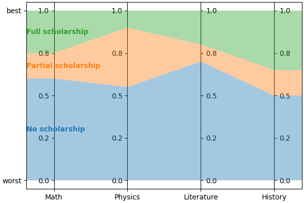
Let’s continue on the scholarship example. Let’s say there a three levels: “no scholarship” (\(C^0\)), “partial scholarship” (\(C^1\)) and “full scholarship” (\(C^2\)). To further simplify things without sacrificing the interest of the example, we can consider four criteria: grades in math (\(M\)), physics (\(P\)), literature (\(L\)) and history (\(H\)), all normalized to be between 0 and 1, and forget about age and family income for now.

For clarity, we’ll use \(M\), \(P\), \(L\) and \(H\) as lower indexes instead of \(i\) for criteria. Grades have the form \(x = (x_M, x_P, x_L, x_H) \in X\).

Let’s consider the following NCS model:

• \(b^1 = (b^1_M, b^1_P, b^1_L, b^1_H) = (0.6, 0.55, 0.7, 0.5)\)

• \(\mathcal{F}^1 = \{ \{M, L\}, \{M, H\}, \{P, L\}, \{P, H\}, \{M, P, L\}, \{M, P, H\}, \{M, L, H\}, \{P, L, H\}, \{M, P, L, H\} \}\)

• \(b^2 = (b^2_M, b^2_P, b^2_L, b^2_H) = (0.75, 0.9, 0.8, 0.65)\)

• \(\mathcal{F}^2 = \{ \{M, P, L\}, \{M, P, H\}, \{M, L, H\}, \{P, L, H\}, \{M, P, L, H\} \}\)

You can check that the constraints of NCS models are satisfied:

• \(b^1_i \preccurlyeq_i b^2_i\) for \(i \in \{M, P, L, H\}\)

• \(\mathcal{F}^1\) and \(\mathcal{F}^2\) are up-closed by inclusion

• \(\mathcal{F}^1 \supseteq \mathcal{F}^2\)

The profiles for this model look like this:

The sufficient coalitions for “partial scholarship” (i.e. \(\mathcal{F}^1\)) can be represented by:

\(\mathcal{P}({\{M, P, L, H\}})\) is represented as a lattice where arrows materialize the inclusion relationship (\(\subset\)). Elements of \(\mathcal{F}^1\) are black and others are grey.

And here are the sufficient coalitions for “full scholarship” (i.e. \(\mathcal{F}^2\)):

We can now attribute scholarships to a few students according to this model. We first look for the set of criteria where they get grades above \(b^2\). If this set is in \(\mathcal{F}^2\), then they get a full scholarship. Else, we then check if the set of criteria where they get grades above \(b^1\) is in \(\mathcal{F}^1\). If yes, they get a partial scholarship.

Student	Grades	Above \(b^2\)	In \(\mathcal{F}^2\)	Above \(b^1\)	In \(\mathcal{F}^1\)	Scholarship
A	\((1, 1, 1, 1)\)	\(\{M, P, L, H\}\)	Yes	\(\{M, P, L, H\}\) (unused)	Yes (unused)	Full
B	\((1, 1, 1, 0)\)	\(\{M, P, L\}\)	Yes	\(\{M, P, L\}\) (unused)	Yes (unused)	Full
C	\((0.8, 0.7, 0.85, 0.6)\)	\(\{M, L\}\)	No	\(\{M, P, L, H\}\)	Yes	Partial
D	\((1, 0, 1, 0)\)	\(\{M, L\}\)	No	\(\{M, L\}\)	Yes	Partial
E	\((1, 1, 0, 0)\)	\(\{M, P\}\)	No	\(\{M, P\}\)	No	None

In prose, this model can be formulated as follows:

• students who have excellent grades (above \(b^2\)) in at least three subjects get a full scholarship

• students who have good grades (above \(b^1\)) in at least one scientific subject (\(M\) and \(P\)) and at least one literary subject (\(L\) and \(H\)) get a partial scholarship

• other students get no scholarship

Back to the concepts!

Particular cases

Some particular cases are quite common. They are NCS models with additional constraints, so they are slightly less general, but sufficient in many cases and computationally simpler to learn.

Here are a few that are used in lincs:

\(U^c \textsf{-} NCS\)

A \(U^c \textsf{-} NCS\) model is an NCS model where all \(\mathcal{F}^h\) are the same. This simplification captures the idea that in many cases, the same criteria are sufficient for all categories, and that categories differ by their lower performance profile.

Formal definition

A \(U^c \textsf{-} NCS\) model is an NCS model with the following additional constraint:

• there is a single \(\mathcal{F} \subseteq \mathcal{P}([0..n))\) such that \(\mathcal{F}^h = \mathcal{F}\) for each category \(h \in [1..p)\)

In the previous model example, \(\mathcal{F}^1 \ne \mathcal{F}^2\), so it is not a \(U^c \textsf{-} NCS\) model.

\(1 \textsf{-} U^c \textsf{-} NCS\) a.k.a. MR-Sort

An MR-Sort model is a \(U^c \textsf{-} NCS\) model with the additional simplification that \(\mathcal{F}\) is defined using weights on criteria and a threshold. A coalition is sufficient if the sum of the weights of its criteria is above 1.

It was introduced by Agnès Leroy et al. in Learning the Parameters of a Multiple Criteria Sorting Method.

Formal definition

An MR-Sort model is a \(U^c \textsf{-} NCS\) model with the following additional parameters:

• for each criterion \(i \in [0..n)\):

  • its weight \(w_i \in [0, 1]\)

and the following additional constraint:

• \(\mathcal{F} = \{ S \in \mathcal{P}([0..n)): \sum_{i \in S} w_i \geq 1 \}\)

Again, this definition differs slightly from others in the literature but is formally equivalent, and is used because it matches our implementation more closely.

Example

Let’s consider a simplified form of our previous model example, with only the two categories \(C^0\) and \(C^1\), and the same profile \(b^1\) and sufficient coalitions \(\mathcal{F}^1\) as before. Is it an MR-Sort model? To answer this question, we can try to find weights \(w_M\), \(w_P\), \(w_L\), \(w_H\) such that \(\mathcal{F}^1 = \{ S \in \mathcal{P}(\{M, P, L, H\}): \sum_{i \in S} w_i \geq 1 \}\). This gives us \(|\mathcal{P}(\{M, P, L, H\})| = 16\) equations, among which the following 6 are of interest:

• \(w_M + w_P \lt 1\) (because \(\{M, P\} \notin \mathcal{F}^1\))

• \(w_L + w_H \lt 1\) (because \(\{L, H\} \notin \mathcal{F}^1\))

• \(w_M + w_L \ge 1\) (because \(\{M, L\} \in \mathcal{F}^1\))

• \(w_P + w_L \ge 1\) (because \(\{P, L\} \in \mathcal{F}^1\))

• \(w_M + w_H \ge 1\) (because \(\{M, H\} \in \mathcal{F}^1\))

• \(w_P + w_H \ge 1\) (because \(\{P, H\} \in \mathcal{F}^1\))

Summing the first two equations gives \(w_M + w_P + w_L + w_H \lt 2\), and summing the last four gives \(w_M + w_P + w_L + w_H \ge 2\), so there is no solution, and that model is not MR-Sort.

By contrast, the coalitions \(\mathcal{F}^2\) of the previous model example can be expressed using the following weights: \(w_M = 0.4\), \(w_P = 0.4\), \(w_L = 0.4\), \(w_H = 0.4\): coalitions of at most two criteria have weights sums less than 1, and coalitions of at least 3 criteria have weights sums greater than 1.

Intuitively, MR-Sort models can express slightly fewer differences in the importance of criteria than \(U^c \textsf{-} NCS\) models.

Classification accuracy

The success of a learning algorithm can be measured according to two main metrics:

• the duration of the learning (the quicker the better)

• the accuracy of the learned model (the higher the better)

The accuracy of the learned model is defined as the portion of alternatives that are classified by the learned model into the same category as in the learning set.

Real-world data is often noisy: the learning set often contains inconsistencies that prevents it from being the result of an NCS classification. In those cases, it’s impossible to find an NCS model with 100% accuracy, but it’s still useful to find a model with a good accuracy.

Here is a summary of the learning methods implemented in lincs:

Algorithm	Model learned	Typical duration	Result on success	Result on failure
SAT (by coalitions or by separation)	\(U^c \textsf{-} NCS\)	Quickest	A model with 100% accuracy	Nothing
WPB heuristic	MR-Sort	Intermediate	A model with accuracy above specified goal	The best model so far
max-SAT (by coalitions or by separation)	\(U^c \textsf{-} NCS\)	Longest	A model with maximum accuracy	(no failure)

Note that none of these algorithms produces “the” model: there is no such thing as a single best model.

The SAT approaches are often the quickest, but when a model with 100% accuracy doesn’t exist, they simply fail to produce anything.

The WPB approach can be configured to produce its “best model so far” if it takes too long to reach the specified accuracy goal.

Provided enough computing resources (time and memory), the max-SAT approaches always reach the best possible accuracy, but can be longer than practical.

The SAT and max-SAT approaches were implemented using their description by Ali Tlili, Khaled Belahcène et al. in Learning non-compensatory sorting models using efficient SAT/MaxSAT formulations. Note that they were introduced in previous articles, and that this article conveniently gathers them in a single place.

The WPB heuristic was described by Olivier Sobrie in his Ph.D thesis. It was originaly implemented in Python by Olivier Sobrie. Emma Dixneuf, Thibault Monsel and Thomas Vindard then provided a sequential C++ implementation of Sobrie’s heuristic, and lincs provides two parallel implementations (using OpenMP and CUDA).

Synthetic data

It’s not always practical to use real-world data when developing a new learning algorithm, so one can use synthetic data instead. In that approach, one specifies the problem and provides a pre-known model. They then generate pseudo-random alternatives classified according to that original model, and use them as a training set to learn a new model. Finally, they compare how close the learned model behaves to the original one to evaluate the quality of the learning algorithm.

lincs provides ways to generate synthetic pseudo-random problems, models and training sets (noisy or clean).

Next

If you haven’t done so yet, we recommend you now follow our “Get started” guide.